pyfssa Tutorial
Preamble
from __future__ import division
# configure plotting
%config InlineBackend.rc = {'figure.dpi': 300, 'savefig.dpi': 300, \
                            'figure.figsize': (6, 6 / 1.6), 'font.size': 12, \
                            'figure.facecolor': (1, 1, 1, 0)}
%matplotlib inline
import itertools

from cycler import cycler
import matplotlib as mpl
import matplotlib.pyplot as plt
import numpy as np
import seaborn as sns
/home/sorge/repos/sci/pyfssa/.devenv35/lib/python3.5/site-packages/matplotlib/__init__.py:872: UserWarning: axes.color_cycle is deprecated and replaced with axes.prop_cycle; please use the latter.
  warnings.warn(self.msg_depr % (key, alt_key))
import fssa
A mock scaling function
In this tutorial, we will demonstrate the pyfssa routines with a mock scaling function
def mock_scaling_f(x):
    """Mock scaling function"""
    return np.exp(-(x + 1.0)**2)
x = np.linspace(-4.0, 2.0, num=200)
fig, ax = plt.subplots()
ax.plot(x, mock_scaling_f(x), label=r'$\tilde{f}(x)$', rasterized=True)
ax.set_xbound(x.min(), x.max())
ax.set_ybound(0.0, 1.1)
ax.set_xlabel(r'$x$')
ax.legend()
plt.show()
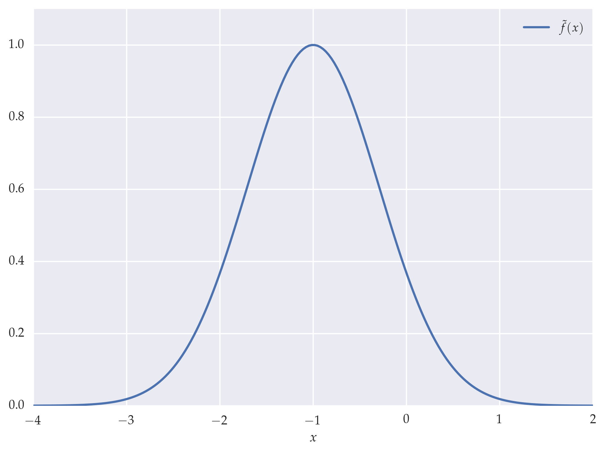
Figure: Mock scaling function \(\tilde{f}(x) = e^{-(x+1)^2}\)
Precisely mocking scaled data
We generate mock observations \(a_{L,\varrho}\) according to the finite-size scaling
with mock exponents \(\nu = \frac{5}{2}, \zeta=\frac{3}{2}\) and \(\rho_c = \frac{1}{2}\).
def mock_scaled_data(l, rho, rho_c=0.5, nu=2.5, zeta=1.5):
    """Generate scaled data from mock scaling function"""
    return np.transpose(
        np.power(l, zeta / nu) *
        mock_scaling_f(
            np.outer(
                (rho - rho_c), np.power(l, 1 / nu)
            )
        )
    )
rhos = np.linspace(-0.5, 0.8, num=200)
ls = np.logspace(1, 3, num=5).astype(np.int)
# system sizes
ls
array([ 10, 31, 100, 316, 1000])
# Define colors
palette = sns.cubehelix_palette(
    n_colors=ls.size, start=2.0, rot=0.35, gamma=1.0, hue=1.0, light=0.6, dark=0.2,
)
sns.palplot(palette)

# Generate precisely mocked scaled data
a = mock_scaled_data(ls, rhos)
fig, ax = plt.subplots()
ax.set_prop_cycle(cycler('color', palette))
for l_index, l in enumerate(ls):
    ax.plot(
        rhos, a[l_index, :],
        '.',
        label=r'${}$'.format(l),
        rasterized=True,
    )
ax.set_xbound(rhos.min(), rhos.max())
ax.set_xlabel(r'$\rho$')
ax.legend(title=r'$L$', loc='upper left')
plt.show()
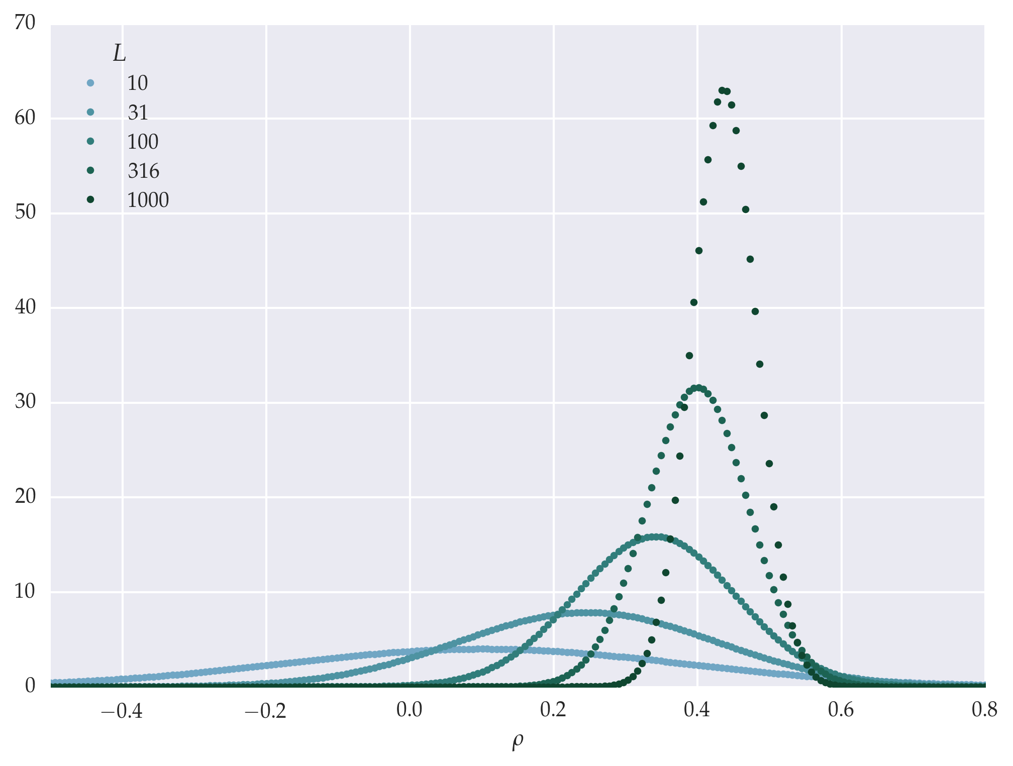
Figure: Mocked raw data, precisely sampled from the scaling function and de-scaled.
Achieving data collapse with the mock data
Our mock data we now want to scale with the fssa.scaledata routine. We compare the quality of the data collapse of several values for the critical exponents, numerically and graphically.
# Put some relative error bars on the precise data
da = a * 0.1
rho_c = np.tile(0.5, (3, 3))
nu = np.tile(2.5, (3, 3))
zeta = np.tile(1.5, (3, 3))
rho_c[0, :] = [0.25, 0.5, 0.75]
nu[1, :] = [2.0, 2.5, 3.0]
zeta[2, :] = [1.0, 1.5, 2.0]
# re-scale data (manually)
scaled_data = list()
quality = list()
for i in range(3):
    my_scaled_data = list()
    my_quality = list()
    for j in range(3):
        my_scaled_data.append(
            fssa.scaledata(
                ls, rhos, a, da,
                rho_c[i, j], nu[i, j], zeta[i, j]
            )
        )
        my_quality.append(fssa.quality(*my_scaled_data[-1]))
    scaled_data.append(my_scaled_data)
    quality.append(my_quality)
# plot manually re-scaled data
fig, axes = plt.subplots(
    nrows=3, ncols=3, squeeze=True,
    #figsize=(8, 7),
    sharex=True, sharey=True,
)

for (i, j) in itertools.product(range(3), range(3)):
    ax = axes[i, j]
    ax.set_prop_cycle(cycler('color', palette))
    my_scaled_data = scaled_data[i][j]
    for l_index, l in enumerate(ls):
        ax.plot(
            my_scaled_data.x[l_index, :], my_scaled_data.y[l_index, :],
            '.',
            label=r'${}$'.format(l),
            rasterized=True,
        )
    ax.set_xbound(-5, 2)
    if i == 0:
        ax.set_title(
            r'$\rho_c = {}$'.format(rho_c[i, j]),
            position=(0.25, 0.65),
        )
    elif i == 1:
        ax.set_title(
            r'$\nu = {}$'.format(nu[i, j]),
            position=(0.25, 0.65),
        )
    elif i == 2:
        ax.set_title(
            r'$\zeta = {}$'.format(zeta[i, j]),
            position=(0.25, 0.65),
        )
    if i == 2:
        ax.set_xlabel(r'$x$')
        ax.set_xticks([-4, -2, 0, ])
    if j == 0:
        ax.set_yticks([0, 1, 2, 3, 4, 5])
    ax.text(
        0.1, 0.5,
        r'$S={:.1f}$'.format(quality[i][j]),
        transform=ax.transAxes,
    )

plt.show()
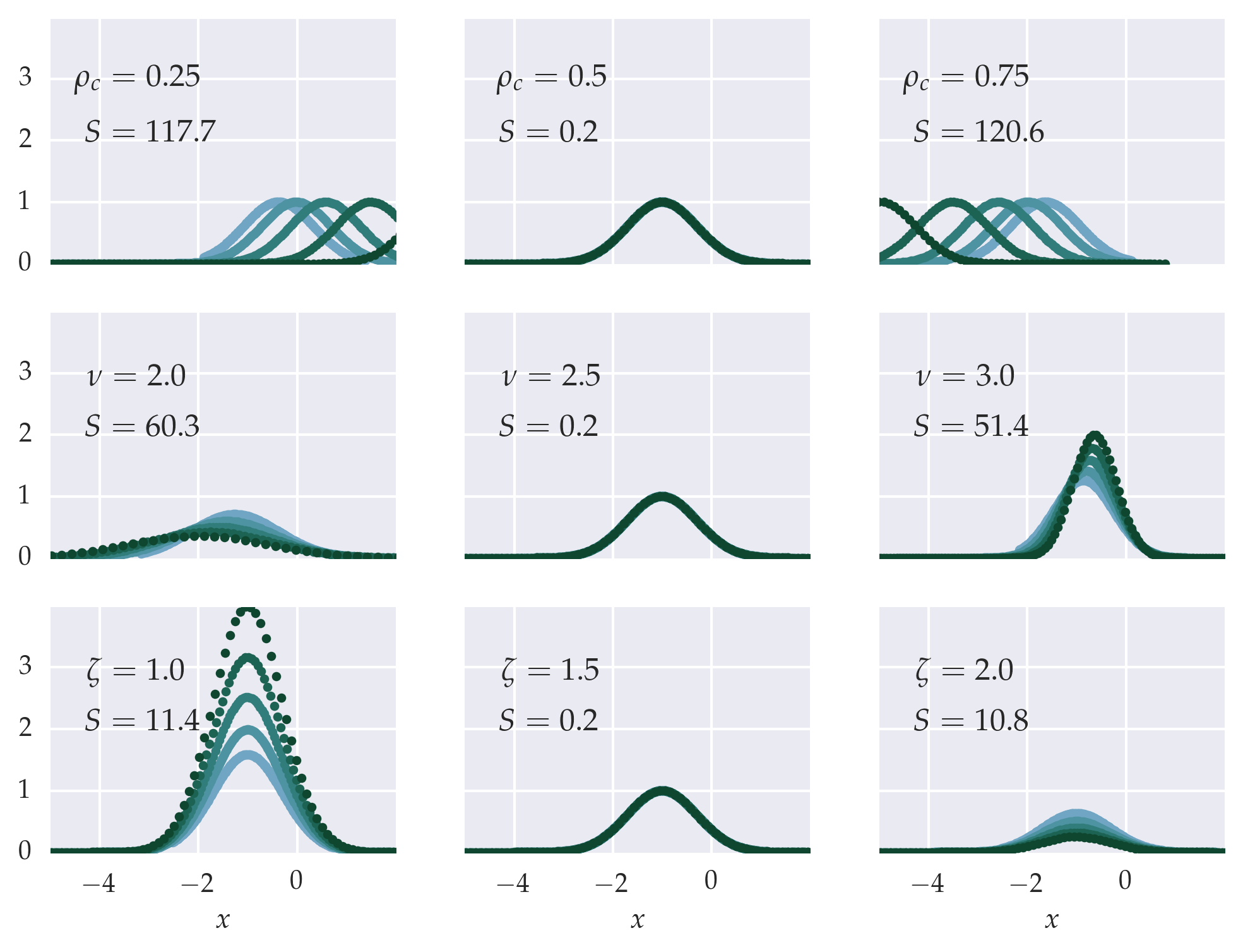
Figure: Scaling the mock data with varying exponents. The true exponents are in the middle column as the critical parameter \(\rho_c = \frac{1}{2}\) and \(\nu = \frac{5}{2}\), \(\zeta = \frac{3}{2}\), as signified by the data collapse onto the single master curve and the quality-of-fit \(S\) (smaller is better).
Auto-scaling the mock data
Now that we have an idea of the approximate range of the exponents, we employ the fssa.autoscale function to algorithmically determine accurate values and their errors.
ret = fssa.autoscale(ls, rhos, a, da, 0.4, 1.8, 2.2)
ret
      message: 'Optimization terminated successfully.'
          rho: 0.49998651420931617
           nu: 2.5029600101429974
          fun: 0.17526760830186447
         zeta: 1.4952017139156362
        varco: array([[  8.73865721e-06,   3.63193042e-05,  -2.29670016e-05],
      [  3.63193042e-05,   1.92714401e-04,  -2.37981434e-04],
      [ -2.29670016e-05,  -2.37981434e-04,   4.25360904e-03]])
final_simplex: (array([[ 0.49998651,  2.50296001,  1.49520171],
      [ 0.50050506,  2.5043243 ,  1.50331343],
      [ 0.50051167,  2.50509256,  1.49581337],
      [ 0.49998317,  2.50366177,  1.50347298]]), array([ 0.17526761,  0.17641794,  0.17700658,  0.18406708]))
       errors: array([ 0.00295612,  0.01388216,  0.0652197 ])
            x: array([ 0.49998651,  2.50296001,  1.49520171])
        dzeta: 0.065219698289192385
       status: 0
      success: True
          dnu: 0.013882161249126912
          nit: 42
         nfev: 74
         drho: 0.0029561219887328798
auto_scaled_data = fssa.scaledata(ls, rhos, a, da, ret.rho, ret.nu, ret.zeta)
# critical exponents and errors, quality of data collapse
print(ret.rho, ret.drho)
print(ret.nu, ret.dnu)
print(ret.zeta, ret.dzeta)
print(ret.fun)
0.499986514209 0.00295612198873
2.50296001014 0.0138821612491
1.49520171392 0.0652196982892
0.175267608302
fig, ax = plt.subplots()
ax.set_prop_cycle(cycler('color', palette))
ax.plot(
    auto_scaled_data.x.T, auto_scaled_data.y.T,
    '.',
)
ax.set_xbound(-4, 2)
ax.set_xlabel(r'$x$')
plt.show()
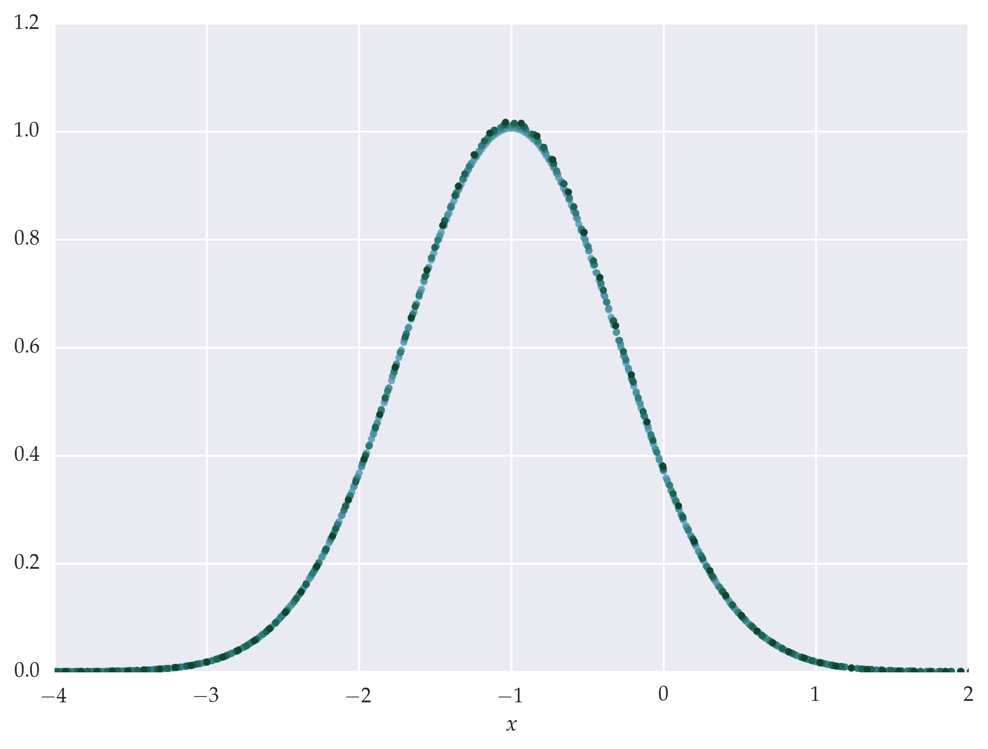
Figure: Auto-scaling with pyfssa leads to data collapse of the mock data onto the original scaling function.
Auto-scaling noisy mock data
noisy_a = a + a * 0.015 * np.random.standard_normal(a.shape)
noisy_ret = fssa.autoscale(ls, rhos, noisy_a, da, 0.4, 1.8, 2.2)
noisy_ret
      message: 'Optimization terminated successfully.'
          rho: 0.49979612592224609
           nu: 2.5018014976584313
          fun: 0.19734634712706023
         zeta: 1.5036671478584973
        varco: array([[  9.53621435e-06,   3.91298047e-05,  -2.84083526e-05],
      [  3.91298047e-05,   2.09742160e-04,  -2.92044395e-04],
      [ -2.84083526e-05,  -2.92044395e-04,   4.95583290e-03]])
final_simplex: (array([[ 0.49979613,  2.5018015 ,  1.50366715],
      [ 0.50029063,  2.50273293,  1.50083439],
      [ 0.500754  ,  2.50594539,  1.49960779],
      [ 0.50059354,  2.50430462,  1.51015554]]), array([ 0.19734635,  0.19844804,  0.20223142,  0.20427539]))
       errors: array([ 0.00308808,  0.01448248,  0.07039768])
            x: array([ 0.49979613,  2.5018015 ,  1.50366715])
        dzeta: 0.070397676820182428
       status: 0
      success: True
          dnu: 0.014482477694416154
          nit: 41
         nfev: 72
         drho: 0.0030880761568600015
noisy_auto_scaled_data = fssa.scaledata(
    ls, rhos, noisy_a, da, noisy_ret.rho, noisy_ret.nu, noisy_ret.zeta
)
fig, ax = plt.subplots()
ax.set_prop_cycle(cycler('color', palette))
ax.plot(
    noisy_auto_scaled_data.x.T, noisy_auto_scaled_data.y.T,
    '.',
)
ax.set_xbound(-4, 2)
ax.set_xlabel(r'$x$')
plt.show()
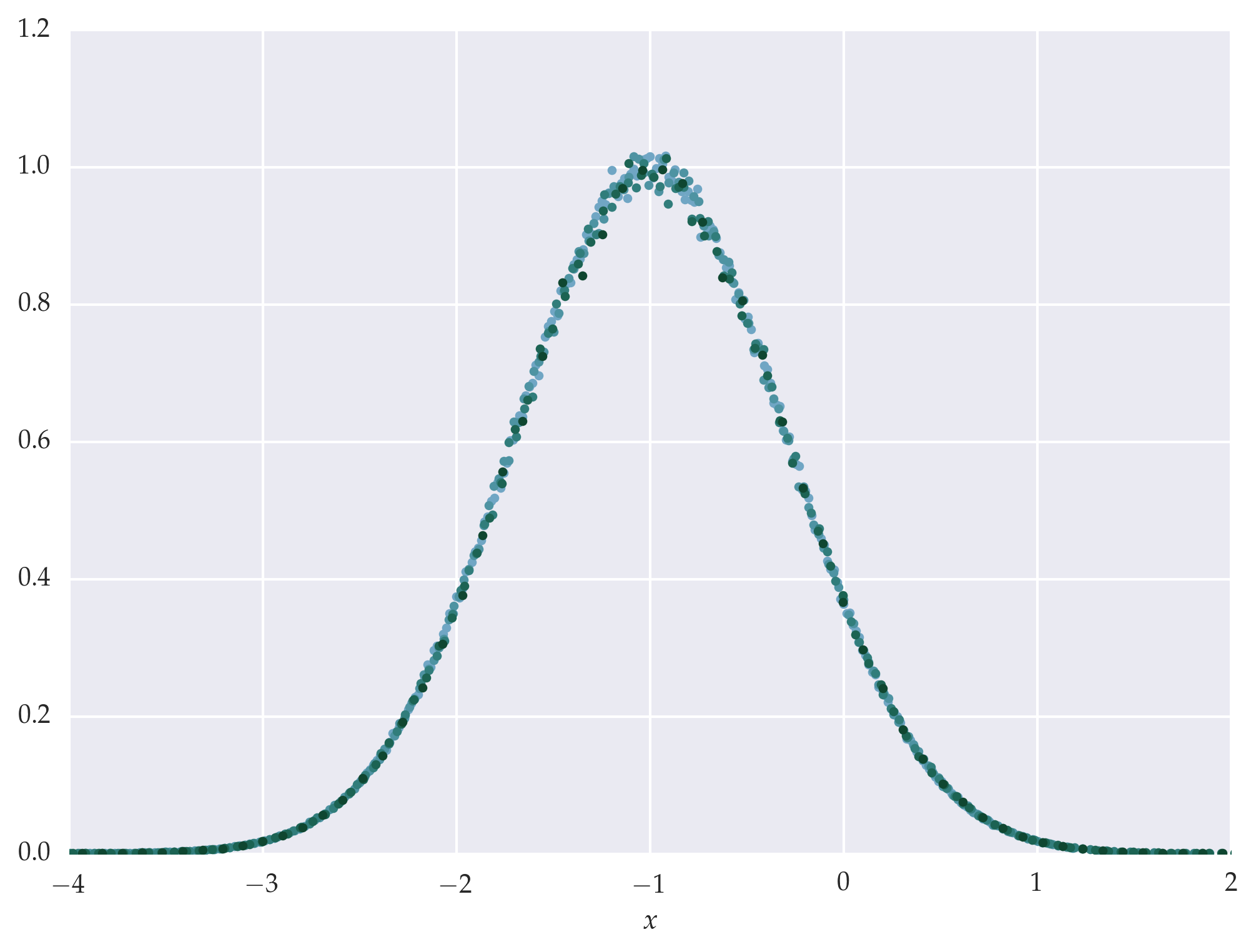
Figure: Auto-scaling with pyfssa leads to data collapse of the noisy mock data onto the original scaling function.
